Logistic Regression
This name could make many colleges confused. In fact, it is a linear model for binary classification tasks. Let’s think about how computer could classify two people according to their features(such as height, weight, hair length, et.al). Of course we should use statistical method combining with lots of data. LR is hereinafter referred to as the “Logistic Regression”. LR is one linear model to do classification tasks. It first calculate a result according to a linear model such as \(y=w^T∗x\). Then it regularizes \(y\) into space \([0,1]\). And 0, 1 represent two classes. At last, if \(y\) is closer to 0, then it belongs to 0. Otherwise 1.
OK. Comes with the question, how do we regularize \(y\)? And why we convert it to space \([0,1]\) not \([−1,1]\)?
Explanation with commercial concepts
Suppose we have the classification task, predict one customer whether to buy a product according to some features, such as salary, gender, age, et.al. Suppose one customer buy product’s probability is \(p\), then \(1-p\)is the un-buy probability. Define \(q = \frac{p}{1-p}\), then \(q \in (0, +\infty)\). Now we should find a function to fit \(q\). When pp is 0, it means the people don’t want to buy anything, now \(q\) is 0. When \(p\) increase a bit, \(q\) nearly didn’t increase. When one has strong feeling to buy, \(q\) increases rapidly. At last it tends to infinity. The exponential function is the best to describe this characteristics. So we use \(e^y\) (refer to following picture)to fit \(q\). Such that \(q=\frac{p}{1-p}=e^y\)
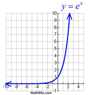
Then, \(p=\frac{1}{1+e^y}\). This is the \(sigmoid\) function, and this function is the core of logistic regression.
Statistical Explanation
The above explanation is very rigorous. Now from statistic point of view, we can think the binary classification problem as n Bernoulli experiments. That is \(X \sim B(n, \theta)\), then \(p(y=1|\theta) = \theta\), \(p(y=0|\theta)=1-\theta\).
So that \[ p(y|\theta) = \theta^{y} (1-\theta)^{1-y} \] And the likelihood function is: \[ L = \prod_{i=1}^n p^{(i)} \] According to maximum likelihood estimation: \(max(L)\) is equals to \(max(\log(L))\)
so the objective is: \[ obj = max(\sum_{i=1}^n(\log p^{(i)})) \]
\[ obj = max(\sum_{i=1}^n (y^{(i)}\log\theta + (1-y^{(i)})\log(1-\theta))) \]
\[ obj = max(\sum_{i=1}^n (\log(1-\theta) + y^{(i)} \log\frac{\theta}{1-\theta})) \]
where \(y^{(i)} = W^T x^{(i)}\)
Generalized Linear Model
Above section has done the statistical explanation, but there are two unknown parameters: \(W^T\) and \(\theta\). Actually we want the probability \(\theta\) could be associated with \(x\) and \(W^T\). For detailed explanation, please refer to my previous blog General Linear Models