Data Lake

Big data has envolved about 10 years from its born, currently the most popular big data solution is not Hadoop, but Data Lake. It includes data ingestion, data storage, processing&analysis and inference.

A data lake is a centralized repository that allows you to store all your structured and unstructured data at any scale. You can store your data as-is, without having to first structure the data, and run different types of analytics—from dashboards and visualizations to big data processing, real-time analytics, and machine learning to guide better decisions.

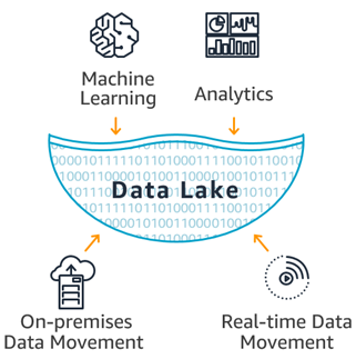
Before big data, we must have heard decision support system, data warehouse and business intelligence. These tools are mainly for struetured data analysis, such as OLAP workloads. But for big data, not only structure data, but semi-structure and non-structure data, these tool are not that suitable(high cost or limited computation/storage). At the time, Google has lanched their data processing infrastructure -- MapReduce which used for processing log files or web pages. Its great capability and cost-effective have made it become the market darling. Utill now the big data platform based on Hadoop, such as cloudera, MapR are also the most popular on-premise big data solutions.

Actually data lake combine the functionality of DWH and Hadoop. It has some key difference between DWH. Let's explore the difference between data lake and DWH.

A data warehouse is a database optimized to analyze relational data coming from transactional systems and line of business applications. The data structure, and schema are defined in advance to optimize for fast SQL queries, where the results are typically used for operational reporting and analysis. Data is cleaned, enriched, and transformed so it can act as the “single source of truth” that users can trust.

Table 1: DWH, Data Lake comparision

Data lake is based on Hadoop and envolved a lot. For Hadoop, it is based on the theory of data locality which made it cost-effective and popular. But now, the hardware price have decreased a lot. We can use the same price to afford a SSD which has very high read disk speed. Due to the data locality, computation and storage are tight coupling which lead the poor scalability. For example, I have encountered a real case which use on-premise Hadoop cluster as the big data platform. For last one year, its computation usage is about 15%. But now the storage usage rate is about 70%, which means they must to scale out their cluster for fulfill their storage requirements. If they scale out the cluster, the cup usage must be even lower. So the key difference between data lake and Hadoop cluster is computation and storage de-coupling. Except that data lake have better scalability, if on cloud the storage and computation would be infinite.

Welcome to Hexo! This is your very first post. Check documentation for more info. If you get any problems when using Hexo, you can find the answer in troubleshooting or you can ask me on GitHub.

Quick Start

Create a new post

1

$ hexo new "My New Post"

More info: Writing

Run server

1

$ hexo server

More info: Server

Generate static files

1

$ hexo generate

More info: Generating

Deploy to remote sites

1

$ hexo deploy

More info: Deployment

Tree Model in Machine Learning

Hope somebody have heard about Decision Tree, CART, Random Forest, GBDT, et.al. Actually, all of those algorithms are based on Tree. How could tree would help computes to do classification or regression tasks? Let’s explore it:

Define Task

Before exploring all of those tree models, let’s define the task which we would handle by using above algorithms.

Classification Task

Suppose, we want to predict whether a person like playing computer games according to gender, age, occupation, et.al.

Then the problem set is: Given \(X\in F_{m\times n}, Y \in {like, dislike}\) to predict person whether like computer games.

Regression Task

Nowadays in China, the house pricing is the most concerned topic. Suppose we have a lot of house parameters such as size, the distance btw mall, et.al. Then we need to predict houses’ price according to historic data.

Then the problem set: Given \(X\in F_{m\times n}, Y\in R_{1\times n}\) to build a model to predict house’s price according to \(X,Y\)

Decision Tree

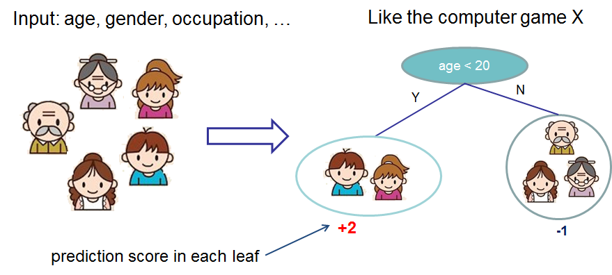
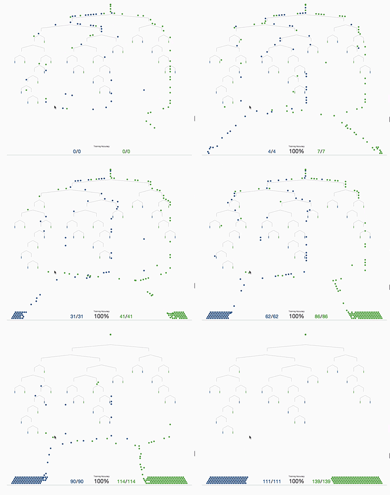
Let’s look at the following picture(copy from xgboost):

Then you would know the process of decision tree. We need to choose a feature to split the whole data sets until the tree node cannot to split. And the critical problem is how to choose the splitting feature at each step.

Impurity

Suppose the whole dataset is impure due to there are too many classes(like, dislike). At each step, we need to choose a feature which could increase the purity after splitting the dataset according to the selected feature. Because the split node would contain small classes.

• Information Entropy

  Entropy is used to define the confusion degree of a system. In information theory, Shannon used it to define the information. The entropy is bigger, the information is more. We could use it to define the impurity. The entropy is bigger, the impurity is bigger. \[ Entropy(X) = \sum_{i=0}^c -p_i \log p_i \] \(p_i = \frac{num\ of \ class\ i}{total\ num}\)

• Gini Coefficient

  Gini coefficient is used to define the income equality. It is bigger then the income is more inequality. So could also use it to define the impurity. The gini index is bigger, the impurity is bigger. \[ Gini(X) = 1- \sum_{i=1}^{c}p_i^2 \] , \(p_i\) is the same as above.

Information/Purity Gain

Above we have talked about how to define the impurity. So we split the dataset based on the feature which could most increase the dataset’s purity. No matter entropy or gini index, after splitting they would decrease. So the information gain is: \[ Gain(X, f) = Impurity\_before - Impurity\_after \]

\[ Impurity\_after = \sum_{v=1}^V \frac{|D_v|}{|D|} impurity\_of\_v \]

So at each step , we choose the biggest Gain feature to split the tree node until reach some condition(depth, leaf node constriction, et.al.). After the tree built, we could use the model to do classification, just like a marble flow from the root node to leafs. Each leaf represents one class/label.

Note:

• Let’s think about one index feature, such as there 100 sample, then their index feature is 1,2,…,1001,2,…,100 . The index feature would lead to best split. But it is of course not a good choice. Actually Information Gain prefers the more value features.
• How could we deal with numerical features? Bucketing

Conclusion

Now let conclude the decision tree algorithm:

• Compute current impurity (Entropy or Gini Index), impurity_before
• Select a feature and compute the impurity, impurity_after
• Repeat Step 2 for all features
• Compute the information gain for all features
• Select the biggest information gain feature to split current node
• Repeat above steps until cannot be split

Regression Tree

Above we have explored how decision tree do classification tasks. Now we will go through the regression task. Let’s think about the difference between classification and regression. The most important is the class/label. Classification task would have fixed values, but for regression it would be infinity. In decision tree, we could use the fixed classed to compute the impurity and found best split. In regression, how could we split the tree? And how to measure the impurity after splitting?

In regression tree, we often use mean square error (hereinafter is MSE) to measure the impurity. Of course, we could use other variants of MSE, such as mean absolute error(hereinafter MAE), friedman_mse, et.al.

Then when do regression, after data points flowed to leaf nodes, the predicted result is the average label of leaf node. That is: \(result=average(leaf(y))\)

That’s easy!!!

Ensemble Learning

Bias-Variance Decomposition

Define following variables:

• \(E(f;D)\) : error between actual value and predicted value.
• \(f(x;D)\) : predicted value on train set D
• \(f(x)=ED[f(x;D)]\): expectation of \(f(x;D)\) on different datasets
• \(y_D\): label on train set D
• \(y\): actual label of the true distribution for whole data set

For regression, we could decompose \(E(f;D)\) as follows: \[ E(f;D) = E_D[(f(x;D)-f(x))^2] + (f(x)-y)^2 + E_D[(y_D-y)^2] \] So \(var = E_d[(f(x;D)-f(x))^2]\) is the variance caused by the limited train set. And \(noise = E_D[(y_D-y)^2]\)

which caused by data, and we cannot get over it.

\(bias = (f(x) - y)^2\) is the bias between predicted value of model and actual label.

That is: \(E(f;D) = bias + var + noise\)

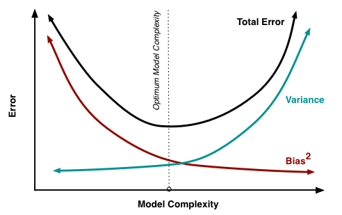
So we could improve our model from two points: bias and var

Bias-variance Trade-off

Intuitively, bias represents the error between model predicted value and the train set’s value. variance indicates the error between train set’s value and the actual value. When bias decreased(model fits train set better), variancewould increase. Because when train more, the data quality could effect accuracy more. We called this is Bias-variance trade-off

Bagging

Bagging is the method which improve models from var point of view. It increases the train data sets’ diversity by sub-sampling both on instances and features. The most popular Tree Model bagging algorithm is Random Forest.

Random Forest & Extremely Randomized Trees

A random forest is a meta estimator that fits a number of decision tree classifiers on various sub-samples of the dataset and use averaging to improve the predictive accuracy and control over-fitting. Please refer to the Bias-variance decomposition in Random Forests to get more about why using more models ensemble could decrease the variance.

Boosting

Until now, we could improve our model’s accuracy by decreasing variance. Are there any methods which could both decrease variance and bias? Of course, boosting could make this dream comes true.

Logistic Regression

This name could make many colleges confused. In fact, it is a linear model for binary classification tasks. Let’s think about how computer could classify two people according to their features(such as height, weight, hair length, et.al). Of course we should use statistical method combining with lots of data. LR is hereinafter referred to as the “Logistic Regression”. LR is one linear model to do classification tasks. It first calculate a result according to a linear model such as \(y=w^T∗x\). Then it regularizes \(y\) into space \([0,1]\). And 0, 1 represent two classes. At last, if \(y\) is closer to 0, then it belongs to 0. Otherwise 1.

OK. Comes with the question, how do we regularize \(y\)? And why we convert it to space \([0,1]\) not \([−1,1]\)?

Explanation with commercial concepts

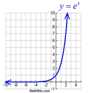
Suppose we have the classification task, predict one customer whether to buy a product according to some features, such as salary, gender, age, et.al. Suppose one customer buy product’s probability is \(p\), then \(1-p\)is the un-buy probability. Define \(q = \frac{p}{1-p}\), then \(q \in (0, +\infty)\). Now we should find a function to fit \(q\). When pp is 0, it means the people don’t want to buy anything, now \(q\) is 0. When \(p\) increase a bit, \(q\) nearly didn’t increase. When one has strong feeling to buy, \(q\) increases rapidly. At last it tends to infinity. The exponential function is the best to describe this characteristics. So we use \(e^y\) (refer to following picture)to fit \(q\). Such that \(q=\frac{p}{1-p}=e^y\)

Then, \(p=\frac{1}{1+e^y}\). This is the \(sigmoid\) function, and this function is the core of logistic regression.

Statistical Explanation

The above explanation is very rigorous. Now from statistic point of view, we can think the binary classification problem as n Bernoulli experiments. That is \(X \sim B(n, \theta)\), then \(p(y=1|\theta) = \theta\), \(p(y=0|\theta)=1-\theta\).

So that \[ p(y|\theta) = \theta^{y} (1-\theta)^{1-y} \] And the likelihood function is: \[ L = \prod_{i=1}^n p^{(i)} \] According to maximum likelihood estimation: \(max(L)\) is equals to \(max(\log(L))\)

so the objective is: \[ obj = max(\sum_{i=1}^n(\log p^{(i)})) \]

\[ obj = max(\sum_{i=1}^n (y^{(i)}\log\theta + (1-y^{(i)})\log(1-\theta))) \]

\[ obj = max(\sum_{i=1}^n (\log(1-\theta) + y^{(i)} \log\frac{\theta}{1-\theta})) \]

where \(y^{(i)} = W^T x^{(i)}\)

Generalized Linear Model

Above section has done the statistical explanation, but there are two unknown parameters: \(W^T\) and \(\theta\). Actually we want the probability \(\theta\) could be associated with \(x\) and \(W^T\). For detailed explanation, please refer to my previous blog General Linear Models

Linear Regression

Linear Regression is the first algorithm when I start to learn machine learning. Before machine learning, I have got in touch with it in statistics. In my memory, linear regression is very simple. And the most important thing is Least Mean Square(hereinafter LMS). But why using LMS to calculate linear regression model? Now we will explore this.

Construct the problem

Given the sample\(X\in R_{m \times n}\) (we always use column vector to represent sample data), \(Y\in R_{1 \times n}\). Suppose \(x\) and \(y\)has the linear relationship, we need to get the model’s parameters \(W \in R_{m \times 1}\). Except that, we would give a \(bias\). So the model would be: \[ Y = W^{T} * X + bias \] For simplicity, we could extend \(X\) to \(R_{m+1 \times n}\). The last row are all 1. Then extend \(W\) to \(R_{m+1 \times n}\), the \(bias\) could be merged to \(W\). Now the model becomes: \[ Y = W^{T} * X \] An the problem is to calculate the unknown item \(W\)

Theory Analysis

Above we have constructed the problem, due to the sample data always more than parameters. So we cannot get a unique result. But we could use optimization to approximate the result: \[ Y^{‘} = W^{T} * X \] , where \[ Y^{‘} \approx Y \] Now the LSM occurred, define\(L = \frac{1}{2} * (Y^{‘} - Y)^2\) , and minimize \(L\) could make \(Y^{'}\) approximates to \(Y\) . The optimization problem is: \(min(L)\).

Statistical Explanation

From statistical point of view, suppose\(y = y^{‘} + \epsilon\), where \(\epsilon\) is the error. In statistic, we define error is Gaussian distribution, by normalization we could get:\(\epsilon \sim N(0,\delta)\) . So, \[ p(\epsilon|W,x) = \frac{1}{\sqrt{2\pi}\delta} \exp(-\frac{\epsilon^2}{2\delta^2}) = \frac{1}{\sqrt{2\pi}\delta} \exp(-\frac{(y-W^Tx)^2}{2\delta^2}) \] For point \(i\), \(p(ϵ(i)|W,x(i))=p(y(i)|W,x(i))\), so the likelihood function: \[ L(W) = \prod_{i=1}^{n} p(y^{(i)} | W, x^{(i)}) \]

\[ \log{L(W)} = \sum_{i=1}^m p(y^{(i)} | x^{(i)},W) = -m\log{\sqrt{2\pi}\delta} - \sum_{i=1}^m \frac{(y^{(i)} - W^Tx^{(i)})^2}{2\delta^2} \]

According to max likelihood approximation: \[ obj = max(\log L(W)) \] so as to, \[ obj = \min{(\sum_{i=1}^m (y^{(i)} - W^Tx^{(i)})^2)} \] This is the same as Least Mean Square.

Solve the Optimization Problem

In optimization, the gradient decent is the most common used algorithm. It just like people to find a fastest way to get down a hillside. This person would stop to try every directions around him. If one way led to the fastest down way at current location, he would choose it. He would repeat above methods until arrived the destination.

OK. In math, gradient is the fastest rising direction. So we could use negative gradient as the fasted decrease direction. At each step, we compute the gradient of the objective function. Then update the unknown parameters as: \[ W = W - \eta * gradient(obj) \] In detail, for the j-th parameter \(W_j\) of \(W\) , the update rule is: \[ W_j = W_j - \eta * \frac{\partial(obj)}{\partial(x_j^{(i)})} \]

\[ W_j = W_j - \eta * (W^TX^{(i)} - y^{(i)})x^{(i)}_j \]

For all sample data, the update rule is to sum all the gradient: \[ W_j = W_j - \sum_{i=1}^{n}\eta * (W^TX^{(i)} - y^{(i)})x^{(i)}_j \]

线性模型 – Generalize Linear Models

所谓的GLMs是一类机器学习算法，其中最小二乘线性回归（LMS）以及逻辑回归（LR）都是GLMs的一个特例。

线性模型的特性

1. 指数分布族 – The exponential family

   所有GLMs的分布律都可以写成如下的指数分布族：\(p(y;\eta) = b(y)exp(\eta^TT(y) - a(\eta))\)

   其中\(\eta\)被称为自然参数或者规范参数， \(T(y)\) 被称为充分统计量，\(a(\eta)\) 是对数分量函数。

2. 构建GLM的假设条件

   • \(y|x;\theta \sim ExponetialFamily(\eta)\)

   • 给定\(x\)，我们的目标是预测\(T(y)\)的期望值。即希望通过假设函数 \[ h_{\theta}(x) \] 预测的结果满足 \[ h_\theta(x) = E[T(y)|x] \]

   • 自然参数\(\eta\) 与 \(x\) 线性相关，即\(\eta = \theta^Tx\)

线性模型实例

下面我们介绍一些线性模型的实例，比如我们常见的线性回归，逻辑回归以及Softmax回归多分类器。

1. 线性回归

   线性回归是一种进行连续值预测的常用方法。假设有\(m\)个样本,每个样本包含\(n\)个特征，即\(X\in R^{m,n}\)，那么回归预测的问题可以描述成 \[ y^{(i)} = \theta^T * x^{(i)} + \epsilon^{(i)} \] 其中\(\theta\)为待拟合的线性模型的权重，\(\epsilon(i)\)为拟合误差。

   假设各个样本的拟合误差独立同分布于（IID）正态分布，即\(\epsilon^{(i)} \sim N(\mu,\delta^2)\) . 假设\(\mu = 0\)(可以通过正则化来达到)，那么 \[ p(\epsilon^i) = \frac{1}{\sqrt{2\pi}\delta}\exp{-\frac{(\epsilon^{(i)})^2}{2\delta^2}} \]

   \[ p(y^{(i)} | x^{(i)},\theta) = \frac{1}{\sqrt{2\pi}\delta}\exp{-\frac{(y^{(i)} - \theta^T*x^{(i)})^2}{2\delta^2}} \]

   那么，该分布的似然函数为: \[ L(\theta) = \prod_{i=1}^m p(y^{(i)} | x^{(i)},\theta) \]

   \[ \log{L(\theta)} = \sum_{i=1}^m p(y^{(i)} | x^{(i)},\theta) = -m\log{\sqrt{2\pi}\delta} - \sum_{i=1}^m \frac{(y^{(i)} - \theta^Tx^{(i)})^2}{2\delta^2} \]

   为了使得线性模型能够得到较好的拟合效果,即最大似然估计: \[ \max{(\log{L(\theta)})} \] 结合上式，即 \[ \min{(\sum_{i=1}^m (y^{(i)} - \theta^Tx^{(i)})^2)} \] 其中无论\(\delta\)如何取值都与问题求解无关。 那么最终的拟合过程，变成了最小二乘问题。

2. 逻辑回归

   逻辑回归是一种二分类问题，假设给你m个样本，每个样本\(n\)个特征，并且所有样本有两个类别，假设是{0,1}。假设样本服从二项分布，即 \[ p(y=1|\phi) = \phi, p(y=0|\phi) = 1- \phi \] 那么 \[ p(y|\phi) = \phi^y(1-\phi)^{1-y} \]

   \[ p(y|\phi) = \exp{(y\log{\phi} + (1-y)\log{(1-\phi)})} \]

   \[ p(y|\phi) = \exp{(y\log{\frac{\phi}{1-\phi}} + \log{(1-\phi)})} \]

   构建GLM得到： \[ T(y) = y, b(y) = 1, \eta = \log{\frac{\phi}{1-\phi}}, \phi = \frac{1}{1+e^{\eta}}, a(\eta) = \log{(1+e^{\eta})} \] 又 \[ \eta^{(i)} = \theta^T * x^{(i)} \] 所以 \[ \phi^{(i)} = \frac{1}{1+e^{-(\theta^T x^{(i)})}} \] 同时，为了求解拟合参数\(\theta\).参考线性回归的求解过程：

   • 求解似然函数：\(L(\theta) = \prod_{i=1}^{m}((\phi^{(i)})^{y^{(i)}} (1-\phi^{(i)})^{(1-y^{(i)})})\)

   • 对似然函数变形：\(l(\theta) = \log{L(\theta)} = \sum_{i=1}^{m}(y^{(i)}\log{\phi^{(i)}}+(1-y^{(i)})\log{(1-\phi^{(i)})})\)

   • 求解变形后的似然函数的最大值，梯度下降求解。每一步迭代的梯度为： \[ \frac{\partial{(l(\theta))}}{\partial{\theta_j}} = (y\frac{1}{\phi} + (1-y)\frac{1}{1-\phi}) \phi(1-\phi)x_j \]

     \[ \frac{\partial{(l(\theta))}}{\partial{\theta_j}} = (y - \phi)x_{j} \]

3. Softmax回归

   Softmax Regression主要用于解决多分类问题，假设 \[ y\in \{1,2,3,…,k\} \] 用于表示样本的类别。

   \(\phi_i\) 表示样本属于第\(i\)类的概率，即\(p(y=i;\phi) = \phi_i\)

   由于\(\sum_{i=1}^{k}\phi_i = 1\), 所以可以令\(\phi_{k} = 1-\sum_{i=1}^{k-1}\phi_i\)

   为了使得多项分布能够用指数函数族描述，在此引入\(T(y)\),其中 \[ T(1) = \left(\begin{array}{c} 1 \\ 0 \\ 0 \\ \vdots \\ 0 \end{array} \right), T(2) = \left(\begin{array}{c} 0 \\ 1 \\ 0 \\ \vdots \\ 0 \end{array} \right), \ldots, T(k-1) = \left(\begin{array}{c} 0 \\ 0 \\ 0 \\ \vdots \\ 1 \end{array} \right), T(k) = \left(\begin{array}{c} 0 \\ 0 \\ 0 \\ \vdots \\ 0 \end{array} \right) \] 那么\(T(y) \neq y, T(y) \in R^{k-1}\)。且\((T(y))_i = 1\{y=i\}\) ，其中\(1\{.\}=1\) when · is true.

   那么\(E[(T(y))_i] = p(y=i) = \phi_i\) \[ p(y;\phi) = \phi_1^{1\{y=1\}}\phi_2^{1\{y=2\}}\ldots\phi_k^{1\{y=k\}} \]

   \[ p(y;\phi) = \exp({1\{y=1\}}\log\{\phi_1\}+\ldots+{1\{y=k\}}\log\{\phi_k\}) \]

   \[ p(y;\phi) = \exp({1\{y=1\}}\log\{\phi_1\}+\ldots+(1-\sum_{i=1}^{k-1}{1\{y=i\}})\log\{\phi_k\}) \]

   \[ p(y;\phi) = \exp(\sum_{i=1}^{k-1}{1\{y=i\}}\log\{\phi_i\}+\ldots+(1-\sum_{i=1}^{k-1}{1\{y=i\}})\log\{\phi_k\}) \]

   \[ p(y;\phi) = \exp(\sum_{i=1}^{k-1}{1\{y=i\}}\log\{\phi_i/\phi_k\}+\ldots+\log{\phi_k}) \]

   \[ p(y;\phi) = \exp(\sum_{i=1}^{k-1}{(T(y))_i}\log\{\phi_i/\phi_k\}+\ldots+\log{\phi_k}) \]

   \[ p(y;\eta) = b(y)exp(\eta^TT(y) - a(\eta)) \]

   得到$b(y)=1, = (\begin{array}{c} (_1/_k) \ (_2/_k) \ (_3/k) \ \ ({k-1}/_k) \end{array} ) \(, 其中\)a() = -(_k)$

   link function(\(\eta\)为分布律的函数)：\(\eta_i = \log(\phi_i/\phi_k)\)

   response function(分布律为\(\eta\)的函数，也称为softmax函数)：\(\phi_i = e^{\eta_i}/\sum_{j=1}^k{e^{\eta_j}}\)

   又：\(\eta_i=\theta_i^Tx\)

   得：\(\phi_i = \exp(\theta_i^Tx)/\sum_{j=1}^k{\exp(\theta_j^Tx)}\)

   那么假设函数： \[ h_{\theta}(x) = E[T(y)|x;\theta] = \left(\begin{array}{c} \phi_1 \\ \phi_2 \\ \phi_3 \\ \vdots \\ \phi_{k-1} \end{array} \right) = \left(\begin{array}{c} \frac{\exp(\theta_1^Tx)}{\sum_{j=1}^k{\exp(\theta_j^Tx)}} \\ \frac{\exp(\theta_2^Tx)}{\sum_{j=1}^k{\exp(\theta_j^Tx)}} \\ \frac{\exp(\theta_3^Tx)}{\sum_{j=1}^k{\exp(\theta_j^Tx)}} \\ \vdots \\ \frac{\exp(\theta_{k-1}^Tx)}{\sum_{j=1}^k{\exp(\theta_j^Tx)}} \end{array} \right) \] 似然函数为： \[ l(\theta) = \sum_{i=1}^{m}\log(p(y^{(i)}|x^{(i)};\theta)) = \sum_{i=1}^{m}\prod_{l=1}^k(\frac{\exp(\theta_l^Tx^{(i)})}{\sum_{j=1}^k{\exp(\theta_j^Tx^{(i)})}})^{1\{y^{(i)}=l\}} \] 最终求解该似然函数的最优解可以得到整个模型的最优解及其对应的模型。

Step by Step to fulfill softmax classification for MNIST dataset

Step1: Load sample data set

加载MNIST样本数据

1
2

from tensorflow.examples.tutorials.mnist import input_data
mnist = input_data.read_data_sets("MNIST_data/", one_hot=True)

注：在执行上述代码时如果遇到file not gzip file错误，是由于下载的数据有问题。去修改源文件[Where tensorflow located]/local/lib/python2.7/site-packages/tensorflow/contrib/learn/python/learn/datasets/mnist.py, 将SOURCE_URL换成：

1 2	> SOURCE_URL = 'http://yann.lecun.com/exdb/mnist/' >

Step2: Construct GLM(Softmax)

构造假设函数（Softmax分类模型）：\(y = h_{\theta}(x) = softmax(W*x + b)\)

1
2
3
4
5

import tensorflow as tf
x = tf.placeholder(tf.float32, [None, 784])
W = tf.Variable(tf.zeros([784, 10]))
b = tf.Variable(tf.zeros([10]))
y = tf.nn.softmax(tf.matmul(x, W) + b)

Step3: Train GLM(Softmax)

求解假设函数的最优值，构造最优化问题目标函数：\(H_{y_i^{‘}}(y) = H_{y_i^{‘}}(h_{\theta(x^{(i)}})\)

在此使用交叉熵作为目标函数，即：\(H_{y_i^{‘}}(y) = -\sum_i(y_i^{‘})\log(h_{\theta(x^{(i)})})\)

1
2

y_ = tf.placeholder(tf.float32, [None, 10])
cross_entropy = tf.reduce_mean(-tf.reduce_sum(y_ * tf.log(y), reduction_indices=[1]))

亦可以直接使用tensorflow提供的函数计算cross_entropy = tf.reduce_mean(tf.nn.softmax_cross_entropy_with_logits(labels=y_, logits=y))其中y=W*x+b

定义优化方法（梯度下降）

1

train_step = tf.train.GradientDescentOptimizer(0.5).minimize(cross_entropy)

Tensorflow执行优化过程（随机梯度下降）

1
2
3
4
5

sess = tf.InteractiveSession()
tf.global_variables_initializer().run()
for _ in range(1000):
  batch_xs, batch_ys = mnist.train.next_batch(100)
  sess.run(train_step, feed_dict={x: batch_xs, y_: batch_ys})

Step 4: 模型评估

1
2
3

correct_prediction = tf.equal(tf.argmax(y,1), tf.argmax(y_,1))
accuracy = tf.reduce_mean(tf.cast(correct_prediction, tf.float32))
print(sess.run(accuracy, feed_dict={x: mnist.test.images, y_: mnist.test.labels}))